| Homework Submission Process |
- Create a working directory for all your MUMT 307 homework (i.e., mkdir mumt307)
- Create a subdirectory called "homeworkN" (where N = current homework number)
- Put all necessary files, numbered in accordance with the homework questions, in this directory
- When ready to submit, create a "tarball" or "zip" file of the appropriate homework directory (note the addition of a username): tar -czf homeworkN-username.tgz homeworkN/
- Submit the compressed homework directory or files via myCourses
Collaboration Policy: Students can often learn a great deal from their peers. Feel free to seek help from other students (as well as the instructor and TA) when you are having difficulty. But DO NOT COPY assignments. We expect you to write your own patches and code.
Pd Patch Remarks: Design your interfaces in order to group the elements (i.e., buttons, displays, sliders) in an intuitive way. Verify the implementation of the patch so that default parameters are initialized at load time. Add small comments to help the user get started and to understand how the patch works. Test your patch (before delivering it) as if you were a real user that does not know anything about the way it has been implemented. For example, make a copy in another folder, quit Pd, reload the patch and test it. Design each patch in a small window that can be printed on one page only.
Matlab and C++ Code Remarks: Your Matlab and C++ programs should be easy to read and understand. At the top of each script or program, provide the program name, your name, and information about the program and how to use it. For C++ programs, included a g++ compiler statement that can be used to compile the program in the working directory. In your code, be liberal with comments. Even when a program does not execute properly, partial credit may be given based on comments that show good understanding of the issues and ways to approach the solutions. Use the C++ style guide to uniformly format your code.
| Homework #8 | Due: Thursday, 13 November 2025 at 22:00 |
- Choose a sound to model using modal synthesis. It is best if the object being modeled is excited by striking or plucking and its sound consists of a relatively small number (5-10) of strong resonances (there should be a reasonable sense of pitch to the sound). You will need to obtain a recording of the sound, either from the McGill University Master Samples, the University of Iowa Musical Instrument Samples, Free Sound Samples from wiki.laptop.org, by making a recording yourself, or from another source. Estimate the resonance frequencies, decay rates, and relative gains using the fft functions in Matlab or a spectrum analyzer of your choice. Write a Matlab script that implements a bank of resonant filters to resynthesize the sound (and also show in the script how you performed the parameter estimation). You should also record a "dry" strike sound to use to excite the filters and/or add directly to the resultant sound. Experiment with the parameters to improve the synthesized sound quality. [12 pts]
| Homework #7 | Due: Thursday, 6 November 2025 at 22:00 |
- Read pages 90-95 and 115-139 of Computer Music by Dodge & Jerse.
- Implement the FM Clarinet algorithm (DUR = 0.5 seconds; fc = 900 Hz; fm = 600 Hz [fc : fm ratio of 3 : 2]; IMIN = 2; IMAX = 4) described on pages 125-127 of Computer Music by Dodge & Jerse (note that IMIN and IMAX refer to minimum and maximum modulation index values and that F1 and F2 are envelope functions, with corresponding amplitudes of AMP = 1 and fm * (IMAX-IMIN)). The sound should last for DUR seconds and the envelopes should be triggered once per DUR seconds (they have a "frequency" of one time per DUR). The fundamental frequency and DUR of the resulting sound should be specified at the top of the script. You can start with the FM brass Matlab script demonstrated in bell.m. [5 pts]
- Repeat the previous question using Pd. You can start with the FM brass Pd patch demonstrated in brass.pd. [5 pts]
| Homework #6 | Due: Thursday, 31 October 2025 at 22:00 |
- In Matlab, create a unit impulse signal and use it as input to a Schroeder allpass filter with g = 0.7 and a delay of 357 samples (given by a difference equation of y[n] = -g x[n] + x[n-M] + g y[n-M]). Then use the output of that filter as input to a feedback comb filter specified by the difference equation y[n] = x[n] - 0.95 y[n-1037]. Plot the resulting impulse response and the corresponding magnitude frequency response. [2 pts]
- Choose a continuously excited musical instrument sound (ex., wind or bowed-string instruments) to model using additive synthesis. You will need to obtain a recording of the sound (options include the McGill University Master Samples, the University of Iowa Musical Instrument Samples, Free Sound Samples from wiki.laptop.org, by making a recording yourself, or from another source). A single tone is suggested. Roughly estimate the time-varying resonance frequencies and amplitudes using the Short-Time Fourier Transform (FFTs of sequential segments of the time-domain signal ... see exstft.m example) or the spectrogram function in Matlab. Then resynthesize the sound in either Matlab or Pd using sinusoidal oscillators and the estimated parameters (see addsynth1.m for a simple Matlab example with a single frequency component). Include the original soundfile with your submission, as well as the analysis information you derived from it. You should interpolate the sinusoidal amplitudes and frequencies over time as needed. [10 pts]
Note that piece-wise linear envelopes can be generated in Matlab using the interp1 function as follows:
fs = 44100;                      % sample rate
T = 1/fs;                        % sample period
x = [0 30 700 1000];             % time breakpoints in milliseconds
y = [0.0 1.0 0.8 0.0];           % corresponding amplitude breakpoints at times given by vector x
n = 0:44099;                     % time in samples (1 second at 44.1 kHz)
env = interp1(x, y, 1000*n*T);   % scale the time steps to milliseconds
| Homework #5 | Due: Thursday, 2 October 2025 at 22:00 |
- Write a Matlab script that takes the eguitar.wav sound as input and implements a "Wah" effect. Create a resonance filter whose center frequency varies sinusoidally between 300 and 700 Hz at a rate of 1 Hz. The filter Q should be 5. The filter coefficients will need to be recomputed every sample as the center frequency varies and you will need to invoke the Matlab filter function as [y, zf] = filter(b, a, x, zi) to make sure the filter state is saved between calls. Play the resulting effected sound at the end and use spectrogram( y, 1024, 512, 1024, fs, 'yaxis' ) to view the spectral variation of the time-domain signal y over time.
[10 pts]
- In Pd, use the saw~ object with a frequency of 500 Hz as input and filter it with a lowres~ filter with a Q = 0.9 and fc that varies linearly from 5000 to 100 Hz over 3 seconds. Apply amplitude envelopes to ramp the sound up and down over the first and last 100 milliseconds. A bng object should trigger the start of the sound. Use a spectrograph~ object to display the resulting spectrum over time.
[6 pts]
| Homework #4 | Due: Thursday, 25 September 2025 at 22:00 |
- Read pages 169-219 of Computer Music by Dodge & Jerse.
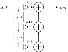
Figure 1: A second-order digital filter.
- Consider the digital filter described by the block diagram in Fig. 1 above:
- Write the difference equation for the filter.
- Using the input signal x[n] = {..., 1, 1, 1, 1, ...}, what is the steady-state gain of the filter at zero frequency?
- Using the input signal x[n] = {..., 1, -1, 1, -1, ...}, what is the steady-state gain of the filter at half the sample rate?
- Is this a FIR or an IIR filter? What general type of filter is it (lowpass, highpass, resonance, shelf, ...)?
- Use the difference equation to calculate the first 5 values of the filter's impulse response (write out the operations by hand).
[3 pts]
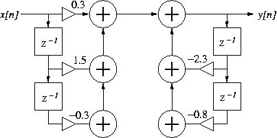
Figure 2: A second-order digital filter.
- Consider the digital filter described by the block diagram in Fig. 2 above:
- Write the difference equation for the filter.
- Use this difference equation to calculate the first 5 values of the filter's impulse response (write out the operations by hand).
- Is the filter stable? Explain your answer.
- In four lines or less (one instruction per line), write Matlab syntax to define the filter and calculate its impulse response (minimum of 50 values).
- Add one more line of Matlab syntax to calculate and plot the filter frequency response (magnitude and phase).
[4 pts]
- Digital Resonance Filters:
- Write Matlab syntax to define a digital resonance filter with a center frequency of 2000 Hz at a sample rate of 44100 Hz (let r = 0.99). The filter gain at the center frequency should be normalized. Verify the design by plotting the filter frequency response.
- Use the Matlab rand function to generate a one-second noise sequence (scale it to a range from -1.0 < x < +1.0 with zero mean) and use this as input to the filter. Use the spectrogram() function to view the spectrum of the resulting filtered noise.
- In Pd, create a patch that implements the same resonance filter using the biquad~ object, with noise~ as input and a spectrograph~ object to view the resulting output signal frequency magnitude response.
- Add a lowres~ object to the same Pd patch, with slider controls for the cutoff frequency (100-4000 Hz) and resonance (0-1). Provide a way to switch between using either the biquad~ or lowres~, with the proper output signal being displayed in the spectrograph~ object.
[4 pts]
| Homework #3 | Due: Thursday, 18 September 2025 at 22:00 |
- Write a matlab script that performs the following operations, all at a sample rate of 44100 Hz:
- Create a wavetable of length N = 1024 samples containing one period of a sinusoid. Add to it 4 more sinusoides with two, three, four and five periods over the same N samples, scaling their amplitudes by factors of 0.5, 0.4, 0.3, and 0.2, respectively. Use the table to produce a sound with a fundamental frequency of 440 Hz for a duration of 2 seconds. You can either interpolate or round the table values at non-integer positions.
- Create a second wavetable of the same length (N = 1024) containing sinusoids with one, three, five, seven and nine periods, scaled in amplitude by 1.0, 0.33, 0.2, 0.14 and 0.11, respectively. Use the table to produce a sound with a fundamental frequency of 440 Hz for a duration of 2 seconds. You can either interpolate or round the table values at non-integer positions.
- Now use both tables, together with the amplitude envelopes shown below, to produce a sound of duration 3 seconds with a fundamental frequency of 550 Hz. Envelope 1 should be applied to the first wavetable above and Envelope 2 should be applied to the second wavetable above. The envelope breakpoints are at times of [0 0.1 1.2 1.8 2.9 3.0]. You can either interpolate or round the table values at non-integer positions.
[12 pts + bonus of 2 pts for correct table interpolation]

- Create a Pd patch that produces the same final 3 second sound as described in the previous question. Use two tabosc4~ objects, with tables created using the sinesum method (see the tabosc4~ help). For the envelopes, use two line~ objects. A single bng object should trigger the start of the sound, with enveloping line segments (up or down) triggered at appropriate times using delay objects.
[6 pts]
| Homework #2 | Due: Thursday, 11 September 2025 at 22:00 |
- Write a matlab script that performs the following operations on the audio file triangle.wav:
- Use the audioread() function to read the audio file data (signal and sample rate) into Matlab variables.
- Play the audio signal using the soundsc() function (which normalizes the signal level and removes any DC offset).
- Plot the magnitude frequency response of the entire signal on a decibel scale. Provide a title and both x- and y-axis labels.
- Plot the spectrogram of the signal, which displays the frequency content of the signal over time. In order to accomplish this, you can use the Matlab function spectrogram(y, WINDOW, NOVERLAP, NFFT, Fs), where WINDOW = 1024, NOVERLAP=512, NFFT=1024, and Fs is the sample rate of the file. Provide a title on the spectrogram.
[5 pts]
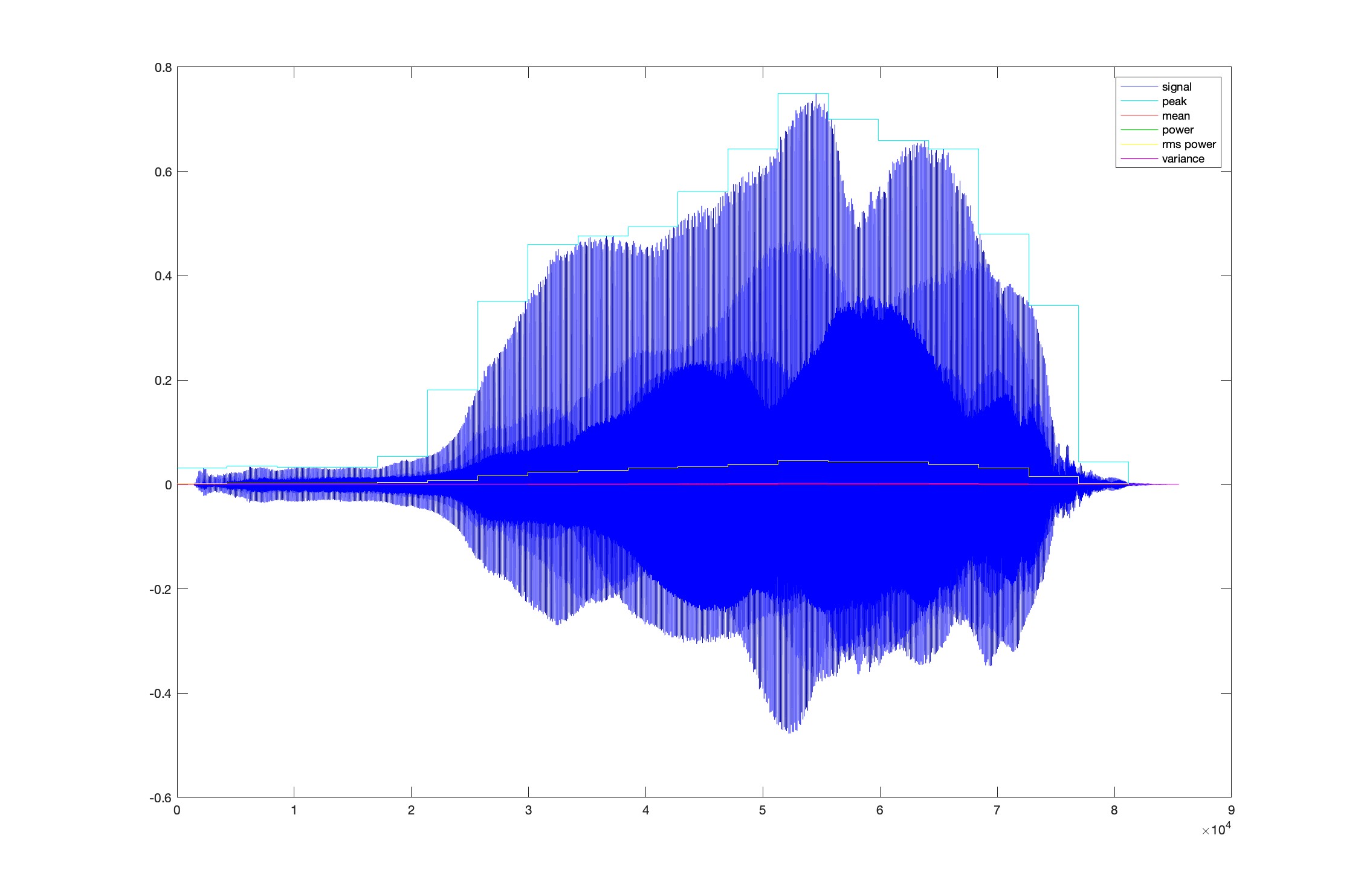
- Write another Matlab script that computes and displays the peak, mean, power, rms power, and variance of the waveform in trumpet.wav. These metrics should be calculated over "blocks" of M samples (define M near the top of your script with a value of 4275) and the plotted metric values should be superposed over the signal as horizontal lines that vary every M samples. Provide a legend in the plot. The Matlab reshape() function can be used to simplify the calculations. The example sinemetrics.m script should provide a good starting point. In the end, the plot should look like the figure below.
[7 pts]
| Homework #1 | Due: Thursday, 4 September 2025 at 22:00 |
- Review chapters 1-3 of Computer Music by Dodge & Jerse, pp. 1-71.
- Read chapter 1 of The Theory and Technique of Electronic Music by Miller Puckette, pp. 1-24.
- Build a Pd patch that simulates a very simple monophonic synthesizer. This synthesizer will include a controlled sound generator and a controlled sound amplifier.
For the generator, the user should be able to select any one of the following three sound sources (only one should sound at a given time): a sinusoid (osc~), noise~ or a soundfile (readsf~). The sinusoid pitch will be controlled using a slider object, with a range of 200-1000 Hz. An openpanel object should be used to select a soundfile and controls should be provided to allow the same file to be repeatedly stopped and started without needing to activate the openpanel again. Controls should also be added to allow continuous looping of the soundfile to be turned on or off. Use a radio button to switch between the generator types and make use of subpatches and the switch~ object so that audio processing is only enabled for a single generator type at a time.
Start and stop buttons should initiate and stop sound production (whichever sound type is currently selected). Use line~ objects to envelope the attack and release, with number boxes to control the attack and release durations in milliseconds in the range of 100-1000 milliseconds. An output gain slider or knob should be used to control the overall sound output level.
Remarks: Think of the implementation in a modular way; design the interface in order to group the parameters into a control front panel (you may use routing objects to clarify the structure of the patch); verify the implementation of the patch so that default parameters are initialized at load time; add small comments to help the user get started and to understand how the patch works; Test your patch (before delivering it) as if you were a real user that does not know anything about the way it has been implemented. For example, make a copy in another folder, quit Pd (or plugdata), reload the patch and test it. Design each patch/subpatch in a small window that can be printed on one page only.
[15 pts]

| ©2004-2025 McGill University. All Rights Reserved.
Maintained by Gary P. Scavone.
|